Visualization
PySwarms implements tools for visualizing the behavior of your swarm.
These are built on top of matplotlib, thus rendering charts that are
easy to use and highly-customizable. However, it must be noted that in
order to use the animation capability in PySwarms (and in matplotlib
for that matter), at least one writer tool must be installed. Some
available tools include: * ffmpeg * ImageMagick * MovieWriter (base)
In the following demonstration, the ffmpeg tool is used. For Linux
and Windows users, it can be installed via:
$ conda install -c conda-forge ffmpeg
In this example, we will demonstrate three plotting methods available on
PySwarms: - plot_cost_history: for plotting the cost history of a
swarm given a matrix - plot_contour: for plotting swarm trajectories
of a 2D-swarm in two-dimensional space - plot_surface: for plotting
swarm trajectories of a 2D-swarm in three-dimensional space
# Import modules
import matplotlib.pyplot as plt
import numpy as np
from matplotlib import animation, rc
from IPython.display import HTML

# Import PySwarms
import pyswarms as ps
from pyswarms.utils.functions import single_obj as fx
from pyswarms.utils.plotters import (plot_cost_history, plot_contour, plot_surface)

# Some more magic so that the notebook will reload external python modules;
# see http://stackoverflow.com/questions/1907993/autoreload-of-modules-in-ipython
%load_ext autoreload
%autoreload 2
The first step is to create an optimizer. Here, we’re going to use
Global-best PSO to find the minima of a sphere function. As usual, we
simply create an instance of its class pyswarms.single.GlobalBestPSO
by passing the required parameters that we will use. Then, we’ll call
the optimize() method for 100 iterations.
options = {'c1':0.5, 'c2':0.3, 'w':0.9}
optimizer = ps.single.GlobalBestPSO(n_particles=50, dimensions=2, options=options)
cost, pos = optimizer.optimize(fx.sphere, iters=100)
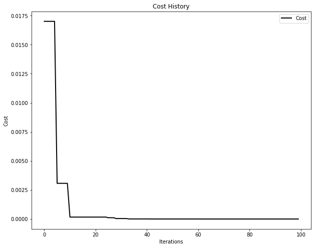
Plotting the cost history
To plot the cost history, we simply obtain the cost_history from the
optimizer class and pass it to the cost_history function.
Furthermore, this method also accepts a keyword argument **kwargs
similar to matplotlib. This enables us to further customize various
artists and elements in the plot. In addition, we can obtain the
following histories from the same class:
- mean_neighbor_history: average local best history of all neighbors throughout optimization
- mean_pbest_history: average personal best of the particles throughout optimization
plot_cost_history(cost_history=optimizer.cost_history)
plt.show()
Animating swarms
The plotters module offers two methods to perform animation,
plot_contour() and plot_surface(). As its name suggests, these
methods plot the particles in a 2-D or 3-D space.
Each animation method returns a matplotlib.animation.Animation class
that still needs to be animated by a Writer class (thus
necessitating the installation of a writer module). For the proceeding
examples, we will convert the animations into an HTML5 video. In such
case, we need to invoke some extra methods to do just that.
# equivalent to rcParams['animation.html'] = 'html5'
# See http://louistiao.me/posts/notebooks/save-matplotlib-animations-as-gifs/
rc('animation', html='html5')
Lastly, it would be nice to add meshes in our swarm to plot the sphere
function. This enables us to visually recognize where the particles are
with respect to our objective function. We can accomplish that using the
Mesher class.
from pyswarms.utils.plotters.formatters import Mesher

# Initialize mesher with sphere function
m = Mesher(func=fx.sphere)
There are different formatters available in the
pyswarms.utils.plotters.formatters module to customize your plots
and visualizations. Aside from Mesher, there is a Designer class
for customizing font sizes, figure sizes, etc. and an Animator class
to set delays and repeats during animation.
Plotting in 2-D space
We can obtain the swarm’s position history using the pos_history
attribute from the optimizer instance. To plot a 2D-contour, simply
pass this together with the Mesher to the plot_contour()
function. In addition, we can also mark the global minima of the sphere
function, (0,0), to visualize the swarm’s “target”.
# Make animation
animation = plot_contour(pos_history=optimizer.pos_history,
                         mesher=m,
                         mark=(0,0))

# Enables us to view it in a Jupyter notebook
HTML(animation.to_html5_video())
Plotting in 3-D space
To plot in 3D space, we need a position-fitness matrix with shape
(iterations, n_particles, 3). The first two columns indicate the x-y
position of the particles, while the third column is the fitness of that
given position. You need to set this up on your own, but we have
provided a helper function to compute this automatically
# Obtain a position-fitness matrix using the Mesher.compute_history_3d()
# method. It requires a cost history obtainable from the optimizer class
pos_history_3d = m.compute_history_3d(optimizer.pos_history)

# Make a designer and set the x,y,z limits to (-1,1), (-1,1) and (-0.1,1) respectively
from pyswarms.utils.plotters.formatters import Designer
d = Designer(limits=[(-1,1), (-1,1), (-0.1,1)], label=['x-axis', 'y-axis', 'z-axis'])

# Make animation
animation3d = plot_surface(pos_history=pos_history_3d, # Use the cost_history we computed
                           mesher=m, designer=d,       # Customizations
                           mark=(0,0,0))               # Mark minima

# Enables us to view it in a Jupyter notebook
HTML(animation3d.to_html5_video())
