Writing your own optimization loop
In this example, we will use the pyswarms.backend module to write our own optimization loop. We will try to recreate the Global best PSO using the native backend in PySwarms. Hopefully, this short tutorial can give you an idea on how to use this for your own custom swarm implementation. The idea is simple, again, let’s refer to this diagram:
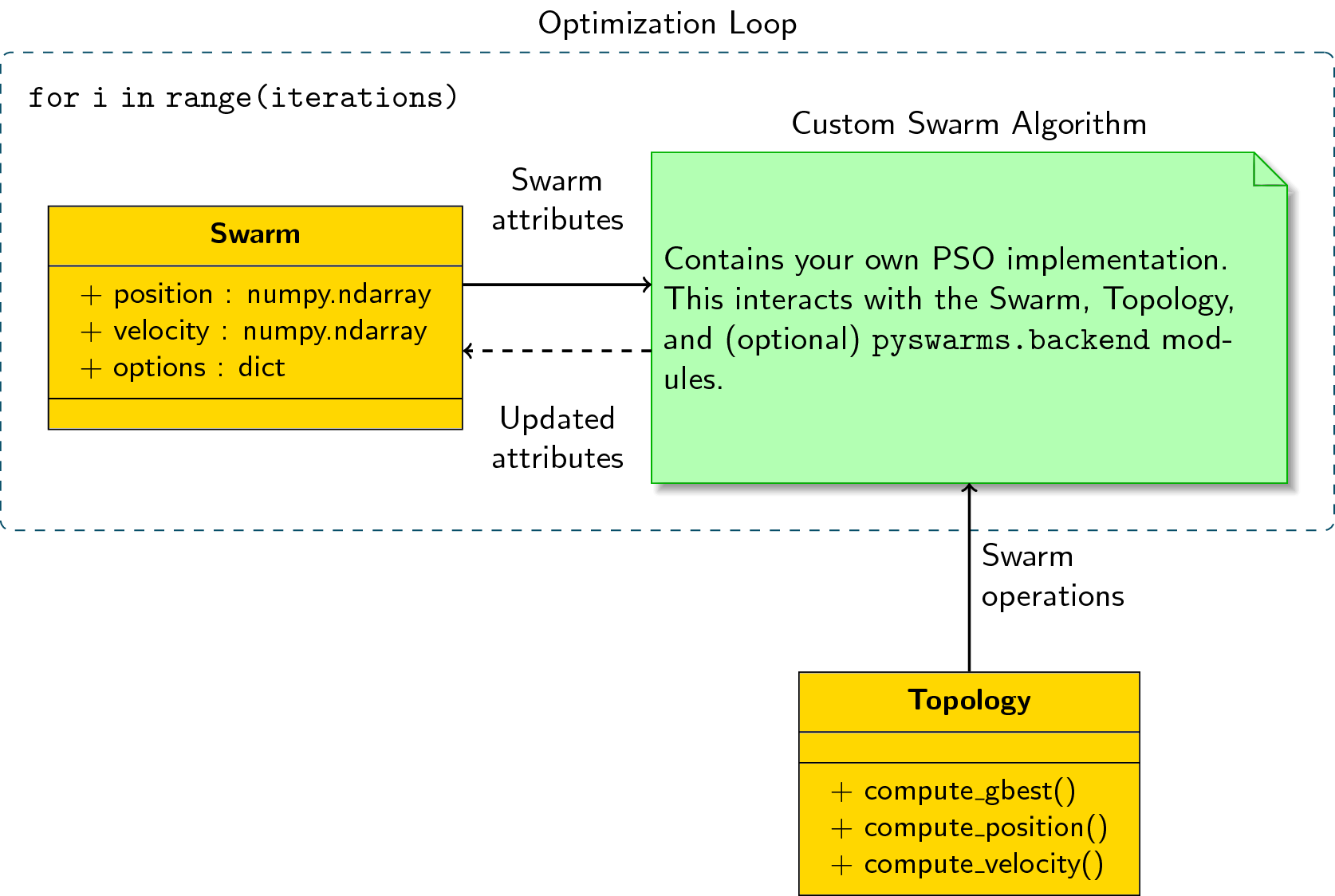
Some things to note: - Initialize a Swarm class and update its attributes for every iteration. - Initialize a Topology class (in this case, we’ll use a Star topology), and use its methods to operate on the Swarm. - We can also use some additional methods in pyswarms.backend depending on our needs.
Thus, for each iteration: 1. We take an attribute from the Swarm class. 2. Operate on it according to our custom algorithm with the help of the Topology class; and 3. Update the Swarm class with the new attributes.
[1]:
# Import modules
import numpy as np

# Import sphere function as objective function
from pyswarms.utils.functions.single_obj import sphere as f

# Import backend modules
import pyswarms.backend as P
from pyswarms.backend.topology import Star

# Some more magic so that the notebook will reload external python modules;
# see http://stackoverflow.com/questions/1907993/autoreload-of-modules-in-ipython
%load_ext autoreload
%autoreload 2
Native global-best PSO implementation
Now, the global best PSO pseudocode looks like the following (adapted from A. Engelbrecht, “Computational Intelligence: An Introduction, 2002):
# Python-version of gbest algorithm from Engelbrecht's book
for i in range(iterations):
    for particle in swarm:
        # Part 1: If current position is less than the personal best,
        if f(current_position[particle]) < f(personal_best[particle]):
            # Update personal best
            personal_best[particle] = current_position[particle]
        # Part 2: If personal best is less than global best,
        if f(personal_best[particle]) < f(global_best):
            # Update global best
            global_best = personal_best[particle]
        # Part 3: Update velocity and position matrices
        update_velocity()
        update_position()
As you can see, the standard PSO has a three-part scheme: update the personal best, update the global best, and update the velocity and position matrices. We’ll follow this three part scheme in our native implementation using the PySwarms backend
Let’s make a 2-dimensional swarm with 50 particles that will optimize the sphere function. First, let’s initialize the important attributes in our algorithm
[2]:
my_topology = Star() # The Topology Class
my_options = {'c1': 0.6, 'c2': 0.3, 'w': 0.4} # arbitrarily set
my_swarm = P.create_swarm(n_particles=50, dimensions=2, options=my_options) # The Swarm Class

print('The following are the attributes of our swarm: {}'.format(my_swarm.__dict__.keys()))
The following are the attributes of our swarm: dict_keys(['position', 'velocity', 'n_particles', 'dimensions', 'options', 'pbest_pos', 'best_pos', 'pbest_cost', 'best_cost', 'current_cost'])
Now, let’s write our optimization loop!
[3]:
iterations = 100 # Set 100 iterations
for i in range(iterations):
    # Part 1: Update personal best
    my_swarm.current_cost = f(my_swarm.position) # Compute current cost
    my_swarm.pbest_cost = f(my_swarm.pbest_pos)  # Compute personal best pos
    my_swarm.pbest_pos, my_swarm.pbest_cost = P.compute_pbest(my_swarm) # Update and store

    # Part 2: Update global best
    # Note that gbest computation is dependent on your topology
    if np.min(my_swarm.pbest_cost) < my_swarm.best_cost:
        my_swarm.best_pos, my_swarm.best_cost = my_topology.compute_gbest(my_swarm)

    # Let's print our output
    if i%20==0:
        print('Iteration: {} | my_swarm.best_cost: {:.4f}'.format(i+1, my_swarm.best_cost))

    # Part 3: Update position and velocity matrices
    # Note that position and velocity updates are dependent on your topology
    my_swarm.velocity = my_topology.compute_velocity(my_swarm)
    my_swarm.position = my_topology.compute_position(my_swarm)

print('The best cost found by our swarm is: {:.4f}'.format(my_swarm.best_cost))
print('The best position found by our swarm is: {}'.format(my_swarm.best_pos))
Iteration: 1 | my_swarm.best_cost: 0.0009
Iteration: 21 | my_swarm.best_cost: 0.0000
Iteration: 41 | my_swarm.best_cost: 0.0000
Iteration: 61 | my_swarm.best_cost: 0.0000
Iteration: 81 | my_swarm.best_cost: 0.0000
The best cost found by our swarm is: 0.0000
The best position found by our swarm is: [3.30572365e-19 2.93696483e-19]
Of course, we can just use the GlobalBestPSO implementation in PySwarms (it has boundary support, tolerance, initial positions, etc.):
[4]:
from pyswarms.single import GlobalBestPSO

optimizer = GlobalBestPSO(n_particles=50, dimensions=2, options=my_options) # Reuse our previous options
optimizer.optimize(f, iters=100)
2019-05-18 15:39:20,737 - pyswarms.single.global_best - INFO - Optimize for 100 iters with {'c1': 0.6, 'c2': 0.3, 'w': 0.4}
pyswarms.single.global_best: 100%|██████████|100/100, best_cost=0.00418
2019-05-18 15:39:21,942 - pyswarms.single.global_best - INFO - Optimization finished | best cost: 0.004177699645933291, best pos: [0.03663518 0.05325001]
[4]:
(0.004177699645933291, array([0.03663518, 0.05325001]))